11 Walkthrough 5: Text analysis with social media data
Abstract
This chapter explores tidying, transforming, visualizing, and analyzing text data. Data scientists in education are surrounded by text-based data sources like word processing documents, emails, and survey responses. Data scientists in education can expand their opportunities to learn about the student experience by adding text mining and natural language processing to their toolkit. Using Twitter data, this chapter shows the reader practical tools for text analysis, including preparing text data, counting and visualizing words, and doing sentiment analysis. The chapter uses Tweets from #tidytuesday, an R learning community, to put these techniques in an education context. Data science tools in this chapter include transforming text into data frames, filtering datasets for keywords, running sentiment analysis and algorithms, and visualizing data.
11.2 Functions introduced
sample_n()set.seed()tidytext::unnest_tokens()nrc::get_sentiments()tidytext::inner_join()
11.5 Chapter overview
The ability to work with many kinds of datasets is one of the great features of doing data science with programming. So far we’ve analyzed data in .csv files, but that’s not the only way data is stored. If we can learn some basic techniques for analyzing text, we increase the number of places we can find information to learn about the student experience.
In this chapter, we focus on analyzing textual data from Twitter. We focus on this particular data source because we think it is relevant to a number of educational topics and questions, including how newcomers learn to visualize data. In addition, Twitter data is complex and includes not only information about who posted a tweet (and when—and a great deal of additional information (see (Michael W. Kearney et al., 2023))), but also the text of the tweet. This makes it especially well–suited for exploring the uses of text analysis, which is broadly part of a group of techniques involving the analysis of text as data—Natural Language Processing (often abbreviated NLP) (Hirschberg & Manning, 2015).
We note that while we focused on #tidytuesday because we think it exemplifies the new kinds of learning-related data that a data science toolkit allows an analyst to try to understand, we also chose this because it is straightforward to access data from Twitter, and - due to the presence of an interactive Shiny application—it is particularly easy to access data on #tidytuesday. While this chapter dives deeply into the analysis of the text of tweets, Appendix B elaborates on a number of techniques for accessing data from Twitter—including data from #tidytuesday—and Chapter 12 explores the nature of the interactions that take place between individuals through #tidytuesday.
11.5.1 Background
When we think about data science in education, our minds tends to go data stored in spreadsheets. But what can we learn about the student experience from text data? Take a moment to mentally review all the moments in your work day that you generated or consumed text data. In education, we’re surrounded by it. We do our lessons in word processor documents, our students submit assignments online, and the school community expresses themselves on public social media platforms. The text we generate can be an authentic reflection of reality in schools, so how might we learn from it?
Even the most basic text analysis techniques will expand your data science toolkit. For example, you can use text analysis to count the number of key words that appear in open-ended survey responses. You can analyze word patterns in student responses or message board posts.
Analyzing a collection of text is different from analyzing large numerical datasets because words don’t have agreed upon values the way numbers do. The number 2 will always be more than 1 and less than 3. The word “fantastic”, on the other hand, has multiple ambiguous levels of degree depending on interpretation and context.
Using text analysis can help to broadly estimate what is happening in the text. When paired with observations, interviews, and close review of the text, this approach can help education staff learn from text data. In this chapter, we’ll learn how to count the frequency of words in a dataset and associate those words with common feelings like positivity or joy.
We’ll show these techniques using a dataset of tweets. We encourage you to complete the walkthrough, then reflect on how the skills learned can be applied to other texts, like word processing documents or websites.
11.5.2 Data source
It’s useful to learn text analysis techniques from datasets that are available for download. Take a moment to do an online search for “download tweet dataset” and note the abundance of Twitter datasets available. Since there’s so much, it’s useful to narrow the tweets to only those that help you answer your analytic questions. Hashtags are text within a tweet that act as a way to categorize content. Here’s an example:
RT @CKVanPay: I’m trying to recreate some Stata code in R, anyone have a good resource for what certain functions in Stata are doing? #RStats #Stata
Twitter recognizes any words that start with a “#” as a hashtag. The hashtags “#RStats” and “#Stata” make this tweet conveniently searchable. If Twitter uses search for “#RStats”, Twitter returns all the Tweets containing that hashtag.
In this example, we’ll be analyzing a dataset of tweets that have the hashtag #tidytuesday (https://twitter.com/hashtag/tidytuesday). #tidytuesday is a community sparked by the work of one of the Data Science in Education Using R co-authors, Jesse Mostipak, who created the (related) #r4ds community from which #tidytuesday was created. #tidytuesday is a weekly data visualization challenge. A great place to see examples from past #tidytuesday challenges is an interactive Shiny application (https://github.com/nsgrantham/tidytuesdayrocks).
The #tidytuesday hashtag (search Twitter for the hashtag, or see the results here: http://bit.ly/tidytuesday-search) returns tweets about the weekly TidyTuesday practice, where folks learning R create and tweet data visualizations they made while learning to use tidyverse R packages.
11.5.3 Methods
In this walkthrough, we’ll be learning how to count words in a text dataset. We’ll also use a technique called sentiment analysis to count and visualize the appearance of words that have a positive association. Lastly, we’ll learn how to get more context by selecting random rows of tweets for closer reading.
11.6 Load packages
For this analysis, we’ll be using the {tidyverse}, {here}, and {dataedu} packages. We will also use the {tidytext} package for working with textual data (Robinson & Silge, 2023). As it has not been used previously in the book, you may need to install the {tidytext} package (and—if you haven’t just yet—the other packages), first. For instructions on and an overview about installing packages, see the “Packages” section of the “Foundational Skills” chapter.
Let’s load our packages before moving on to import the data:
11.7 Import data
Let’s start by getting the data into our environment so we can start analyzing it. In Chapter 12 and in Appendix B, we describe how we accessed this data through Twitter’s Application Programming Interface, or API (and how you can access data from Twitter on other hashtags or terms, too).
We’ve included the raw dataset of TidyTuesday tweets in the {dataedu} package. You can see the dataset by typing tt_tweets. Let’s start by assigning the name raw_tweets to this dataset:
11.8 View data
Let’s return to our raw_tweets dataset. Run glimpse(raw_tweets) and notice the number of variables in this dataset. It’s good practice to use functions like glimpse() or str() to look at the data type of each variable. For this walkthrough, we won’t need all 90 variables so let’s clean the dataset and keep only the ones we want.
11.9 Process data
In this section we’ll select the columns we need for our analysis and we’ll transform the dataset so each row represents a word. After that, our dataset will be ready for exploring.
First, let’s use select() to pick the two columns we’ll need: status_id and text. status_id will help us associate interesting words with a particular tweet and text will give us the text from that tweet. We’ll also change status_id to the character data type since it’s meant to label tweets and doesn’t actually represent a numerical value.
tweets <-
  raw_tweets %>%
  #filter for English tweets
  filter(lang == "en") %>%
  select(status_id, text) %>%
  # Convert the ID field to the character data type
  mutate(status_id = as.character(status_id))
Now the dataset has a column to identify each tweet and a column that shows the text that users tweeted. But each row has the entire tweet in the text variable, which makes it hard to analyze. If we kept our dataset like this, we’d need to use functions on each row to do something like count the number of times the word “good” appears. We can count words more efficiently if each row represented a single word. Splitting sentences in a row into single words in a row is called “tokenizing”. In their book Text Mining With R, Silge & Robinson (2017) describe tokens this way:
A token is a meaningful unit of text, such as a word, that we are interested in using for analysis, and tokenization is the process of splitting text into tokens. This one-token-per-row structure is in contrast to the ways text is often stored in current analyses, perhaps as strings or in a document-term matrix.
Let’s use unnest_tokens() from the {tidytext} package to take our dataset of tweets and transform it into a dataset of words.
## # A tibble: 131,232 × 2
##    status_id           word
##    <chr>               <chr>
##  1 1163154266065735680 first
##  2 1163154266065735680 tidytuesday
##  3 1163154266065735680 submission
##  4 1163154266065735680 roman
##  5 1163154266065735680 emperors
##  6 1163154266065735680 and
##  7 1163154266065735680 their
##  8 1163154266065735680 rise
##  9 1163154266065735680 to
## 10 1163154266065735680 power
## # ℹ 131,222 more rows
We use output = word to tell unnest_tokens() that we want our column of tokens to be called word. We use input = text to tell unnest_tokens() to tokenize the tweets in the text column of our tweets dataset. The result is a new dataset where each row has a single word in the word column and a unique ID in the status_id column that tells us which tweet the word appears in.
Notice that our tokens dataset has many more rows than our tweets dataset. This tells us a lot about how unnest_tokens() works. In the tweets dataset, each row has an entire tweet and its unique ID. Since that unique ID is assigned to the entire tweet, each unique ID only appears once in the dataset. When we used unnest_tokens() put each word on its own row, we broke each tweet into many words. This created additional rows in the dataset. And since each word in a single tweet shares the same ID for that tweet, an ID now appears multiple times in our new dataset.
We’re almost ready to start analyzing the dataset! There’s one more step we’ll take—removing common words that don’t help us learn what people are tweeting about. Words like “the” or “a” are in a category of words called “stop words”. Stop words serve a function in verbal communication, but don’t tell us much on their own. As a result, they clutter our dataset of useful words and make it harder to manage the volume of words we want to analyze. The {tidytext} package includes a dataset called stop_words that we’ll use to remove rows containing stop words. We’ll use anti_join() on our tokens dataset and the stop_words dataset to keep only rows that have words not appearing in the stop_words dataset.
Why does this work? Let’s look closer. inner_join() matches the observations in one dataset to another by a specified common variable. Any rows that don’t have a match get dropped from the resulting dataset. anti_join() does the same thing as inner_join() except it drops matching rows and keeps the rows that don’t match. This is convenient for our analysis because we want to remove rows from tokens that contain words in the stop_words dataset. When we call anti_join(), we’re left with rows that don’t match words in the stop_words dataset. These remaining words are the ones we’ll be analyzing.
One final note before we start counting words: Remember when we first tokenized our dataset and we passed unnest_tokens() the argument output = word? We conveniently chose word as our column name because it matches the column name word in the stop_words dataset. This makes our call to anti_join() simpler because anti_join() knows to look for the column named word in each dataset.
11.10 Analysis: counting words
Now it’s time to start exploring our newly cleaned dataset of tweets. Computing the frequency of each word and seeing which words showed up the most often is a good start. We can pipe tokens to the count function to do this:
## # A tibble: 15,334 × 2
## word n
## <chr> <int>
## 1 t.co 5432
## 2 https 5406
## 3 tidytuesday 4316
## 4 rstats 1748
## 5 data 1105
## 6 code 988
## 7 week 868
## 8 r4ds 675
## 9 dataviz 607
## 10 time 494
## # ℹ 15,324 more rowsWe pass count() the argument sort = TRUE to sort the n variable from the highest value to the lowest value. This makes it easy to see the most frequently occurring words at the top. Not surprisingly, “tidytuesday” was the third most frequent word in this dataset.
We may want to explore further by showing the frequency of words as a percent of the whole dataset. Calculating percentages like this is useful in a lot of education scenarios because it helps us make comparisons across different sized groups. For example, you may want to calculate what percentage of students in each classroom receive special education services.
In our tweets dataset, we’ll be calculating the count of words as a percentage of all tweets. We can do that by using mutate() to add a column called percent. percent will divide n by sum(n), which is the total number of words. Finally, will multiply the result by 100.
tokens %>%
count(word, sort = TRUE) %>%
# n as a percent of total words
mutate(percent = n / sum(n) * 100)## # A tibble: 15,334 × 3
## word n percent
## <chr> <int> <dbl>
## 1 t.co 5432 7.39
## 2 https 5406 7.36
## 3 tidytuesday 4316 5.87
## 4 rstats 1748 2.38
## 5 data 1105 1.50
## 6 code 988 1.34
## 7 week 868 1.18
## 8 r4ds 675 0.919
## 9 dataviz 607 0.826
## 10 time 494 0.672
## # ℹ 15,324 more rowsEven at 4,316 appearances in our dataset, “tidytuesday” represents only about 6% of the total words in our dataset. This makes sense when you consider our dataset contains 15,335 unique words.
11.11 Analysis: sentiment analysis
Now that we have a sense of the most frequently appearing words, it’s time to explore some questions in our tweets dataset. Let’s imagine that we’re education consultants trying to learn about the community surrounding the TidyTuesday data visualization ritual. We know from the first part of our analysis that the token “dataviz” (a short name for data visualization) appeared frequently relative to other words, so maybe we can explore that further. A good start would be to see how the appearance of that token in a tweet is associated with other positive words.
We’ll need to use a technique called “sentiment analysis” to get at the “positivity” of words in these tweets. Sentiment analysis tries to evaluate words for their emotional association. If we analyze words by the emotions they convey, we can start to explore patterns in large text datasets like our tokens data.
Earlier we used anti_join() to remove stop words in our dataset. We’re going to do something similar here to reduce our tokens dataset to only words that have a positive association. We’ll use a dataset called the “NRC Word-Emotion Association Lexicon” to help us identify words with a positive association. This dataset was published in a work called Crowdsourcing a Word-Emotion Association Lexicon (Mohammad & Turney, 2013)
We need to install a package called {textdata} to make sure we have the NRC Word-Emotion Association Lexicon dataset available to us. Note that you only need to have this package installed. You do not need to load it with the library(textdata) command.
If you don’t already have it, let’s install {textdata}:
To explore this dataset more, we’ll use a {tidytext} function called get_sentiments() to view some words and their associated sentiment. If this is your first time using the NRC Word-Emotion Association Lexicon, you’ll be prompted to download the NRC lexicon. Respond “yes” to the prompt and the NRC lexicon will download. Note that you’ll only have to do this the first time you use the NRC lexicon.
## # A tibble: 13,872 × 2
##    word        sentiment
##    <chr>       <chr>
##  1 abacus      trust
##  2 abandon     fear
##  3 abandon     negative
##  4 abandon     sadness
##  5 abandoned   anger
##  6 abandoned   fear
##  7 abandoned   negative
##  8 abandoned   sadness
##  9 abandonment anger
## 10 abandonment fear
## # ℹ 13,862 more rows
This returns a dataset with two columns. The first is word and contains a list of words. The second is the sentiment column, which contains an emotion associated with each word. This dataset is similar to the stop_words dataset. Note that this dataset also uses the column name word, which will again make it easy for us to match this dataset to our tokens dataset.
11.11.1 Count positive words
Let’s begin working on reducing our tokens dataset down to only words that the NRC dataset associates with positivity. We’ll start by creating a new dataset, nrc_pos, which contains the NRC words that have the positive sentiment. Then we’ll match that new dataset to tokens using the word column that is common to both datasets. Finally, we’ll use count() to total up the appearances of each positive word.
# Only positive in the NRC dataset
nrc_pos <-
  get_sentiments("nrc") %>%
  filter(sentiment == "positive")

# Match to tokens
pos_tokens_count <-
  tokens %>%
  inner_join(nrc_pos, by = "word") %>%
  # Total appearance of positive words
  count(word, sort = TRUE)

pos_tokens_count
## # A tibble: 642 × 2
## word n
## <chr> <int>
## 1 fun 173
## 2 top 162
## 3 learn 131
## 4 found 128
## 5 love 113
## 6 community 110
## 7 learning 97
## 8 happy 95
## 9 share 90
## 10 inspired 85
## # ℹ 632 more rowsWe can visualize these words nicely by using {ggplot2} to show the positive words in a bar chart. There are 644 words total, which is hard to convey in a compact chart. We’ll solve that problem by filtering our dataset to only words that appear 75 times or more.
pos_tokens_count %>%
  # only words that appear 75 times or more
  filter(n >= 75) %>%
  ggplot(., aes(x = reorder(word, -n), y = n)) +
  geom_bar(stat = "identity", fill = dataedu_colors("darkblue")) +
  labs(
    title = "Count of Words Associated with Positivity",
    subtitle = "Tweets with the hashtag #tidytuesday",
    caption = "Data: Twitter and NRC",
    x = "",
    y = "Count"
  ) +
  theme_dataedu()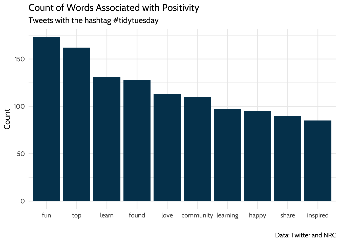
Figure 11.1: Count of Words Associated with Positivity
Note the use of reorder() when mapping the word variable to the x aesthetic. Using reorder() here sorts our x-axis in descending order by the variable n. Sorting the bars from highest frequency to lowest makes it easier for the reader to identify and compare the most and least common words in the visualization.
11.11.2 “Dataviz” and other positive words
Earlier in the analysis we learned that “dataviz” was among the most frequently occurring words in this dataset. We can continue our exploration of TidyTuesday tweets by seeing how many tweets with “dataviz” also had at least one positive word from the NRC dataset. Looking at this might give us some clues about how people in the TidyTuesday learning community view dataviz as a tool.
There are a few steps to this part of the analysis, so let’s review our strategy. We’ll need to use the status_id field in the tweets dataset to filter the tweets that have the word dataviz in them. Then we need to use the status_id field in this new bunch of dataviz tweets to identify the tweets that include at least one positive word.
How do we know which status_id values contain the word “dataviz” and which ones contain a positive word? Recall that our tokens dataset only has one word per row, which makes it easy to use functions like filter() and inner_join() to make two new datasets: one of status_id values that have “dataviz” in the word column and one of status_id values that have a positive word in the word column.
We’ll explore the combinations of “dataviz” and any positive words in our tweets dataset using these three ingredients: our tweets dataset, a vector of status_ids for tweets that have “dataviz” in them, and a vector of status_ids for tweets that have positive words in them. Now that we have our strategy, let’s write some code and see how it works.
First, we’ll make a vector of status_ids for tweets that have “dataviz” in them. This will be used later to identify tweets that contain “dataviz” in the text. We’ll use filter() on our tokens dataset to keep only the rows that have “dataviz” in the word column. Let’s name that new dataset dv_tokens.
## # A tibble: 607 × 2
##    status_id           word
##    <chr>               <chr>
##  1 1116518351147360257 dataviz
##  2 1098025772554612738 dataviz
##  3 1161454327296339968 dataviz
##  4 1110711892086001665 dataviz
##  5 1151926405162291200 dataviz
##  6 1095854400004853765 dataviz
##  7 1157111441419395074 dataviz
##  8 1154958378764046336 dataviz
##  9 1105642831413239808 dataviz
## 10 1108196618464047105 dataviz
## # ℹ 597 more rows
The result is a dataset that has status_id in one column and the word “dataviz” in the other column. We can use $ to extract a vector of status_id for tweets that have “dataviz” in the text. This vector has hundreds of values, so we’ll use head to view just the first ten.
## [1] "1116518351147360257" "1098025772554612738" "1161454327296339968"
## [4] "1110711892086001665" "1151926405162291200" "1095854400004853765"
Now let’s do this again, but this time, we’ll make a vector of status_id for tweets that have positive words in them. This will be used later to identify tweets that contain a positive word in the text. We’ll use filter() on our tokens dataset to keep only the rows that have any of the positive words in the in the word column. If you’ve been running all the code up to this point in the walkthrough, you’ll notice that you already have a dataset of positive words called nrc_pos, which can be turned into a vector of positive words by typing nrc_pos$word. We can use the %in% operator in our call to filter() to find only words that are in this vector of positive words. Let’s name this new dataset pos_tokens.
## # A tibble: 4,885 × 2
##    status_id           word
##    <chr>               <chr>
##  1 1163154266065735680 throne
##  2 1001412196247666688 honey
##  3 1001412196247666688 production
##  4 1001412196247666688 increase
##  5 1001412196247666688 production
##  6 1161638973808287746 found
##  7 991073965899644928  community
##  8 991073965899644928  community
##  9 991073965899644928  trend
## 10 991073965899644928  population
## # ℹ 4,875 more rows
The result is a dataset that has status_id in one column and a positive word from tokens in the other column. We’ll again use $ to extract a vector of status_id for these tweets.
## [1] "1163154266065735680" "1001412196247666688" "1001412196247666688"
## [4] "1001412196247666688" "1001412196247666688" "1161638973808287746"
That’s a lot of status_id, many of which are duplicates. Let’s try and make the vector of status_idsa little shorter. We can use distinct() to get a data frame of status_id, where each status_id only appears once:
Note that distinct() drops all variables except for status_id. For good measure, let’s use distinct() on our dv_tokens data frame too:
Now we have a data frame of status_id for tweets containing “dataviz” and another for tweets containing a positive word. Let’s use these to transform our tweets dataset. First we’ll filter tweets for rows that have the “dataviz” status_id. Then we’ll create a new column called positive that will tell us if the status_id is from our vector of positive word status_ids. We’ll name this filtered dataset dv_pos.
dv_pos <-
  tweets %>%
  # Only tweets that have the dataviz status_id
  filter(status_id %in% dv_tokens$status_id) %>%
  # Is the status_id from our vector of positive word?
  mutate(positive = if_else(status_id %in% pos_tokens$status_id, 1, 0))
Let’s take a moment to dissect how we use if_else() to create our positive column. We gave if_else() three arguments:
status_id %in% pos_tokens$status_id: a logical statement1: the value ofpositiveif the logical statement is true0: the value ofpositiveif the logical statement is false
So our new positive column will take the value 1 if the status_id was in our pos_tokens dataset and the value 0 if the status_id was not in our pos_tokens dataset. Practically speaking, positive is 1 if the tweet has a positive word and 0 if it does not have a positive word.
And finally, let’s see what percent of tweets that had “dataviz” in them also had at least one positive word:
## # A tibble: 2 × 3
##   positive     n  perc
##      <dbl> <int> <dbl>
## 1        0   272 0.450
## 2        1   333 0.550
About 55% of tweets that have “dataviz” in them also had at least one positive word, and about 45% of them did not have at least one positive word. It’s worth noting here that this finding doesn’t necessarily mean users didn’t have anything good to say about 45% of the “dataviz” tweets. We can’t know precisely why some tweets had positive words and some didn’t, we just know that more dataviz tweets had positive words than not. To put this in perspective, we might have a different impression if 5% or 95% of the tweets had positive words.
Since the point of exploratory data analysis is to explore and develop questions, let’s continue to do that. In this last section we’ll review a random selection of tweets for context.
11.11.3 Taking a close read of randomly selected tweets
Let’s review where we are so far as we work to learn more about the TidyTuesday learning community through tweets. So far we’ve counted frequently used words and estimated the number of tweets with positive associations. This dataset is large, so we need to zoom out and find ways to summarize the data. But it’s also useful to explore by zooming in and reading some of the tweets. Reading tweets helps us to build intuition and context about how users talk about TidyTuesday in general. Even though this doesn’t lead to quantitative findings, it helps us to learn more about the content we’re studying and analyzing. Instead of reading all 4,418 tweets, let’s write some code to randomly select tweets to review.
First, let’s make a dataset of tweets that had positive words from the NRC dataset. Remember earlier when we made a dataset of tweets that had “dataviz” and a column that had a value of 1 for containing positive words and 0 for not containing positive words? Let’s reuse that technique, but instead of applying to a dataset of tweets containing “dataviz”, let’s use it on our dataset of all tweets.
pos_tweets <-
  tweets %>%
  mutate(positive = if_else(status_id %in% pos_tokens$status_id, 1, 0)) %>%
  filter(positive == 1)
Again, we’re using if_else to make a new column called positive that takes its value based on whether status_id %in% pos_tokens$status_id is true or not.
We can use slice() to help us pick the rows. When we pass slice() a row number, it returns that row from the dataset. For example, we can select the 1st and 3rd row of our tweets dataset this way:
## # A tibble: 2 × 2
##   status_id           text
##   <chr>               <chr>
## 1 1163154266065735680 "First #TidyTuesday submission! Roman emperors and their …
## 2 1001412196247666688 "My #tidytuesday submission for week 8. Honey production …
Randomly selecting rows from a dataset is great technique to have in your toolkit. Random selection helps us avoid some of the biases we all have when we pick rows to review ourselves.
Here’s one way to do that using base R:
## [1] 4 3 9 8 2Passing sample() a vector of numbers and the size of the sample you want returns a random selection from the vector. Try changing the value of x and size to see how this works.
{dplyr} has a version of this called sample_n() that we can use to randomly select rows in our tweets dataset. Using sample_n() looks like this:
## # A tibble: 10 × 3
## status_id text positive
## <chr> <chr> <dbl>
## 1 1133817727615930369 "@allison_horst @thomas_mock I wonder if there … 1
## 2 1146039959725518848 "Follow @House_of_Honda\n\n\n🔰 This FB6 Is Jus… 1
## 3 988608513663528960 "#TidyTuesday\nI know there must be far easier … 1
## 4 1117623421012205568 "#TidyTuesday #rstats Week 2019-04-09: 50 years… 1
## 5 1029834250063945728 "Following my previous tweet, I took a deep div… 1
## 6 1141050762337882112 "1960: the year owls with extreme-length ears r… 1
## 7 1118668150780907520 "A simple #TidyTuesday submission this week. A … 1
## 8 993149495193100288 "@TheresaWege Great visualization Theresa! Than… 1
## 9 1117692475135520768 "#TidyTuesday inspired by @sil_aarts https://t.… 1
## 10 1143570115864211456 "Had another go at the #tidytuesday bird count … 1That returned ten randomly selected tweets that we can now read through and discuss. Let’s look a little closer at how we did that. We used sample_n(), which returns randomly selected rows from our tweets dataset. We also specified that size = 10, which means we want sample_n() to give us 10 randomly selected rows. A few lines before that, we used set.seed(2020). This helps us ensure that, while sample_n() theoretically plucks 10 random numbers, our readers can run this code and get the same result we did. Using set.seed(2020) at the top of your code makes sample_n() pick the same ten rows every time. Try changing 2020 to another number and notice how sample_n() picks a different set of ten numbers, but repeatedly picks those numbers until you change the argument in set.seed().
11.12 Conclusion
The purpose of this walkthrough is to share code with you so you can practice some basic text-analysis techniques. Now it’s time to make your learning more meaningful by adapting this code to text-based files you regularly see at work. Trying reading in some of these and doing a similar analysis:
- News articles
- Procedure manuals
- Open-ended responses in surveys
There are also advanced text analysis techniques to explore. Consider trying topic modeling (https://www.tidytextmining.com/topicmodeling.html) or finding correlations between terms (https://www.tidytextmining.com/ngrams.html), both described in (Silge & Robinson, 2017).
Finally, if you feel like there is more to analyze where it comes to this particular hashtag, we agree! We use this data set further in the next chapter on social network analysis. Moreover, if you want to collect our own Twitter data, head to Appendix B to read about and consider some potential strategies.