12 Walkthrough 6: Exploring relationships using social network analysis with social media data

Abstract

This chapter explores the use of social network analysis (commonly referred to as SNA). While much of the data that data scientists in education analyze pertains to variables for individuals, some data concerns the relationships between individuals, such as friendship between youth, or advice-seeking on the part of teachers. While such data is common—and often of interest to data scientists—it can be difficult to analyze, in part due to the multiple sources of data (about both individuals’ relations and individuals and the complexity of the relations between individuals. This chapter uses data from the Twitter #tidyuesday network, an R learning community, to demonstrate how such data can be accessed and imported, processed into forms necessary for social network analysis using the {tidygraph} R package, and visualized using the {ggraph} R package.

12.1 Topics emphasized

Transforming data
Visualizing data

12.2 Functions introduced

rtweet::search_tweets()
randomNames::randomNames()
tidyr::unnest()
tidygraph::as_tbl_graph()
ggraph::ggraph()

12.3 Vocabulary

Application Programming Interface (API)
edgelist
edge
influence model
regex
selection model
social network analysis
sociogram
vertex

12.4 Chapter overview

This chapter builds on Walkthrough 5 in Chapter 11, where we worked with #tidytuesday data. In the previous chapter we focused on using text analysis to understand the content of tweets. In this, we chapter focus on the interactions between #tidytuesday participants using social network analysis (sometimes simply referred to as network analysis) techniques.

While social network analysis is increasingly common, it remains challenging to carry out. For one, cleaning and tidying the data can be even more challenging than for most other data sources because net data for social network analysis (or network data) often includes variables about both individuals (such as information students or teachers) and their relationships (whether they have a relationship at all, for example, or how strong or of what type their relationship is). This chapter is designed to take you from not having carried out social network analysis through visualizing network data.

Like the previous chapter, we’ve also included an appendix (Appendix C) to introduce some social network-related ideas for further exploration; these focus on modeling social network processes, particularly, the processes of who chooses (or selects) to interact with whom, and of influence, or how relationships can impact individuals’ behaviors.

You will need a Twitter account to complete all of the code outlined in this chapter in order to access your own Twitter data (through the Twitter Application Interface [API]; see Chapter 11 for an in-depth description of what this means and how to access it).

If you do not have a Twitter account, you can create one and keep it private, or even delete the account once you’re done with this walkthrough. Additionally, you can simply access data that has already been accessed from the Twitter API via the {dataedu} package (as we describe below).

12.4.1 Background

There are a few reasons to be interested in social media. For example, if you work in a school district, you may want to know who is interacting with the content you share. If you are a researcher, you may want to investigate what teachers, administrators, and others do through state-based hashtags (e.g., Joshua M. Rosenberg et al. (2016)). Social media-based data also provides new contexts for learning to take place, like in professional learning networks (Trust et al., 2016).

In the past, if a teacher wanted advice about how to plan a unit or to design a lesson, they would turn to a trusted peer in their building or district (Spillane et al., 2012). Today they are as likely to turn to someone in a social media network. Social media interactions like the ones tagged with the #tidytuesday hashtag are increasingly common in education. Using data science tools to learn from these interactions is valuable for improving the student experience.

12.4.2 Packages

In this chapter, we access data using the {rtweet} package (Michael W. Kearney, 2016). Through {rtweet} and a Twitter account, it is easy to access data from Twitter. We will load the {tidyverse} and {rtweet} packages to get started.

We will also load other packages that we will be using in this analysis, including two packages related to social network analysis (Pedersen, 2022, 2023) as well as one that will help us to use not-anonymized names in a savvy way (Betebenner, 2021). As always, if you have not installed any of these packages before (which may particularly be the case for the {rtweet}, {randomNames}, {tidygraph}, and {ggraph} packages, which we have not yet used in the book), do so using the install.packages() function. More on installing packages is included in the “Packages” section of the “Foundational Skills” chapter.

Let’s load the packages with the following calls to the library() function:

library(tidyverse)
library(rtweet)
library(dataedu)
library(randomNames)
library(tidygraph)
library(ggraph)

12.4.3 Data sources and import

Here is an example of searching the most recent 1,000 tweets, which include the hashtag #rstats. When you run this code, you will be prompted to authenticate your access via Twitter.

rstats_tweets <- 
  search_tweets("#rstats")

You can easily change the search term to other hashtags terms. For example, to search for #tidytuesday tweets, we can replace #rstats with #tidytuesday:

tt_tweets  <- 
  search_tweets("#tidytuesday")

You can find a greater number of tweets by adding a greater value to the n argument of the search_tweets() function, as follows, to collect the most recent 500 tweets:

tt_tweets  <- 
  search_tweets("#tidytuesday", n = 500)

You may notice that the most recent tweets containing the #tidytuesday hashtag are returned. What if you wanted to go further back in time? We’ll discuss this topic in the next section and in Appendix B.

12.4.4 Using an Application Programming Interface (or API)

It’s worth taking a short detour to talk about how you can obtain a dataset spanning a longer period of time. A common way to import data from websites, including social media platforms, is to use something called an Application Programming Interface (API). In fact, if you ran the code above, you just accessed an API!

Think of an API as a special door a home builder made for a house that has a lot of cool stuff in it. The home builder doesn’t want everyone to be able to walk right in and use a bunch of stuff in the house. But they also don’t want to make it too hard because, after all, sharing is caring! Imagine the home builder made a door just for folks who know how to use doors. In order to get through this door, users need to know where to find it along the outside of the house. Once they’re there, they have to know the code to open. And, once they’re through the door, they have to know how to use the stuff inside. An API for social media platforms like Twitter and Facebook are the same way. You can download datasets of social media information, like tweets, using some code and authentication credentials organized by the website.

There are some advantages to using an API to import data at the start of your education dataset analysis. Every time you run the code in your analysis, you’ll be using the API to contact the social media platform and download a fresh dataset. Now your analysis is not just a one-off product, but, rather, is one that can be updated with the most recent data (in this case, Tweets), every time you run it. By using an API to import new data every time you run your code, you create an analysis that can be used again and again on future datasets. However, a key point—and limitation—is that Twitter allows access to their data via their API only for (approximately) the seven most recent days. There are a number of other ways to access older data, though we focus on one way here: having access to the URLs of (or the status IDs for) tweets.

As a result, we used this technique—described in-depth in Appendix B—to collect older (historical) data from Twitter about the #tidytuesday hashtag, using a different function than the one described above (rtweet::lookup_statuses() instead of rtweet::search_tweets()). This was important for this chapter because having access to a greater number of tweets allows us to better understand the interactions between a larger number of the individuals participating in #tidytuesday. The data that we prepared from accessing historical data for #tidytuesday is available in the {dataedu} R package as the tt_tweets dataset, as we describe next.

12.4.4.1 Accessing the data from {dataedu}

Don’t have Twitter or don’t wish to access the data via Twitter? Then, you can load the data from the {dataedu} package (just as we did in the last chapter, Chapter 11), as follows:

tt_tweets <- dataedu::tt_tweets

12.5 View data

We can see that there are many rows for the data:

nrow(tt_tweets)

## [1] 4418

12.6 Methods: process data

Network data requires some processing before it can be used in subsequent analyses. The network dataset needs a way to identify each participant’s role in the interaction. We need to answer questions like: Did someone reach out to another for help? Was someone contacted by another for help? We can process the data by creating an “edgelist”. An edgelist is a dataset where each row is a unique interaction between two parties. Each row (which represents a single relationship) in the edgelist is referred to as an “edge”. We note that one challenge facing data scientists beginning to use network analysis is the different terms that are used for similar (or the same!) aspects of analyses: Edges are sometimes referred to as “ties” or “relations”, but these generally refer to the same thing, though they may be used in different contexts.

An edgelist looks like the following, where the sender (sometimes called the “nominator”) column identifies who is initiating the interaction and the receiver (sometimes called the “nominee”) column identifies who is receiving the interaction:

## # A tibble: 12 × 2
##    sender             receiver          
##    <chr>              <chr>             
##  1 Sielaff, Shelby    el-Radwan, Sumayya
##  2 el-Hashemi, Saabir el-Salim, Sakeena 
##  3 el-Hashemi, Saabir Roberts, Aaron    
##  4 Hughes, Micheal    el-Salim, Sakeena 
##  5 Hughes, Micheal    el-Radwan, Sumayya
##  6 Hughes, Micheal    Lucero, Alana     
##  7 Ohlig, Shelby      Roberts, Aaron    
##  8 Ohlig, Shelby      Sorenson, Michelle
##  9 Ohlig, Shelby      Lucero, Alana     
## 10 Porter, Ryan       Zeigler, Marcel   
## 11 Martin, Angela     Roberts, Aaron    
## 12 Martin, Angela     Zeigler, Marcel

In this edgelist, the sender column might identify someone who nominates another (the receiver) as someone they go to for help. The sender might also identify someone who interacts with the receiver in other ways, like “liking” or “mentioning” their tweets. In the following steps, we will work to create an edgelist from the data from #tidytuesday on Twitter.

12.6.1 Extracting mentions

Let’s extract the mentions. There is a lot going on in the code below; let’s break it down line-by-line, starting with mutate():

mutate(all_mentions = str_extract_all(text, regex)): this line uses a regex, or regular expression, to identify all of the usernames in the tweet (note: the regex comes from this Stack Overflow page (https://stackoverflow.com/questions/18164839/get-twitter-username-with-regex-in-r))
unnest(all_mentions) this line uses a {tidyr} function, unnest() to move every mention to its own line, while keeping all of the other information the same (see more about unnest() here: https://tidyr.tidyverse.org/reference/unnest.html)).

Now let’s use these functions to extract the mentions from the dataset. Here’s how all the code looks in action:

regex <- "@([A-Za-z]+[A-Za-z0-9_]+)(?![A-Za-z0-9_]*\\.)"

tt_tweets <-
  tt_tweets %>%
  # Use regular expression to identify all the usernames in a tweet
  mutate(all_mentions = str_extract_all(text, regex)) %>%
  unnest(all_mentions)

Let’s put these into their own data frame, called mentions.

mentions <-
  tt_tweets %>%
  mutate(all_mentions = str_trim(all_mentions)) %>%
  select(sender = screen_name, all_mentions)

12.6.2 Putting the edgelist together

Recall that an edgelist is a data structure that has columns for the “sender” and “receiver” of interactions. Someone “sends” the mention to someone who is mentioned, who can be considered to “receive” it. To make the edgelist, we’ll need to clean it up a little by removing the “@” symbol. Let’s look at our data as it is now.

mentions

## # A tibble: 2,447 × 2
##    sender  all_mentions    
##    <chr>   <chr>           
##  1 cizzart @eldestapeweb   
##  2 cizzart @INDECArgentina 
##  3 cizzart @ENACOMArgentina
##  4 cizzart @tribunalelecmns
##  5 cizzart @CamaraElectoral
##  6 cizzart @INDECArgentina 
##  7 cizzart @tribunalelecmns
##  8 cizzart @CamaraElectoral
##  9 cizzart @AgroMnes       
## 10 cizzart @AgroindustriaAR
## # ℹ 2,437 more rows

Let’s remove that “@” symbol from the columns we created and save the results to a new tibble, edgelist.

edgelist <- 
  mentions %>% 
  # remove "@" from all_mentions column
  mutate(all_mentions = str_sub(all_mentions, start = 2)) %>% 
  # rename all_mentions to receiver
  select(sender, receiver = all_mentions)

12.7 Analysis and results

Now that we have our edgelist, let’s plot the network. We’ll use the {tidygraph} and {ggraph} packages to visualize the data. We note that network visualizations are often referred to as “sociograms” or a representation of the relationships between individuals in a network. We use this term and the term network visualization interchangeably in this chapter.

12.7.1 Plotting the network

Large networks like this one can be hard to work with because of their size. We can get around that problem by only including some individuals. Let’s explore how many interactions each individual in the network sent by using count():

interactions_sent <- edgelist %>% 
  # this counts how many times each sender appears in the data frame, effectively counting how many interactions each individual sent 
  count(sender) %>% 
  # arranges the data frame in descending order of the number of interactions sent
  arrange(desc(n))

interactions_sent

## # A tibble: 618 × 2
##    sender            n
##    <chr>         <int>
##  1 thomas_mock     347
##  2 R4DScommunity    78
##  3 WireMonkey       52
##  4 CedScherer       41
##  5 allison_horst    37
##  6 mjhendrickson    34
##  7 kigtembu         27
##  8 WeAreRLadies     25
##  9 PBecciu          23
## 10 sil_aarts        23
## # ℹ 608 more rows

618 senders of interactions is a lot! What if we focused on only those who sent more than one interaction?

interactions_sent <- 
  interactions_sent %>% 
  filter(n > 1)

That leaves us with only 349, which will be much easier to work with.

We now need to filter the edgelist to only include these 349 individuals. The following code uses the filter() function combined with the %in% operator to do this:

edgelist <- edgelist %>% 
  # the first of the two lines below filters to include only senders in the interactions_sent data frame
  # the second line does the same, for receivers
  filter(sender %in% interactions_sent$sender,
         receiver %in% interactions_sent$sender)

We’ll use the as_tbl_graph() function, which identifies the first column as the “sender” and the second as the “receiver”. Let’s look at the object it creates:

g <- 
  as_tbl_graph(edgelist)

g

## # A tbl_graph: 267 nodes and 975 edges
## #
## # A directed multigraph with 7 components
## #
## # Node Data: 267 × 1 (active)
##    name           
##    <chr>          
##  1 dgwinfred      
##  2 datawookie     
##  3 jvaghela4      
##  4 FournierJohanie
##  5 JonTheGeek     
##  6 jakekaupp      
##  7 Joseph_Mike    
##  8 barbaravreede  
##  9 geokaramanis   
## 10 R_by_Ryo       
## # ℹ 257 more rows
## #
## # Edge Data: 975 × 2
##    from    to
##   <int> <int>
## 1     1    32
## 2     1    36
## 3     2   120
## # ℹ 972 more rows

We can see that the network now has 267 individuals, all of whom sent more than one interaction. The individuals in a network are often referred to as “nodes” (and this terminology is used in the {ggraph} functions for plotting the individuals—the nodes—in a network). We note that nodes are sometimes referred to as “vertices” or “actors”; like the different names for edges, these generally mean the same thing.

Next, we’ll use the ggraph() function:

g %>%
  # we chose the kk layout as it created a graph which was easy-to-interpret, but others are available; see ?ggraph
  ggraph(layout = "kk") +
  # this adds the points to the graph
  geom_node_point() +
  # this adds the links, or the edges; alpha = .2 makes it so that the lines are partially transparent
  geom_edge_link(alpha = .2) +
  # this last line of code adds a ggplot2 theme suitable for network graphs
  theme_graph()

## Warning: Using the `size` aesthetic in this geom was deprecated in ggplot2 3.4.0.
## ℹ Please use `linewidth` in the `default_aes` field and elsewhere instead.
## This warning is displayed once every 8 hours.
## Call `lifecycle::last_lifecycle_warnings()` to see where this warning was
## generated.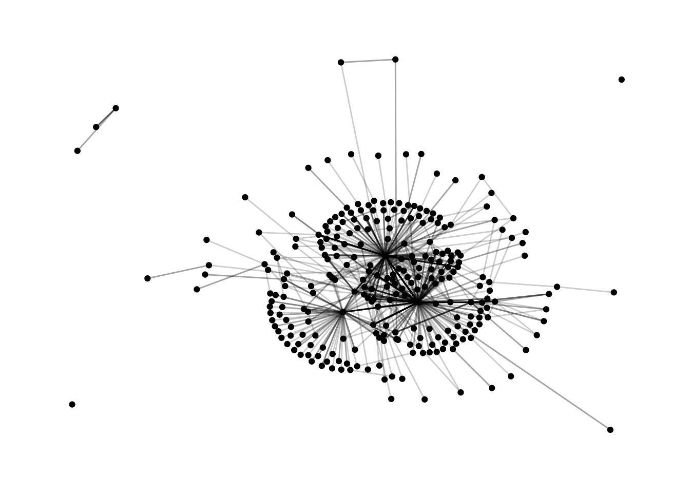

Figure 12.1: Network Graph

Finally, let’s size the points based on a measure of centrality. A common way to do this is to measure how influential an individual may be based on the interactions observed.

g %>% 
  # this calculates the centrality of each individual using the built-in centrality_authority() function
  mutate(centrality = centrality_authority()) %>% 
  ggraph(layout = "kk") + 
  geom_node_point(aes(size = centrality, color = centrality)) +
  # this line colors the points based upon their centrality
  scale_color_continuous(guide = 'legend') + 
  geom_edge_link(alpha = .2) +
  theme_graph()

## Warning in grid.Call(C_stringMetric, as.graphicsAnnot(x$label)): font family
## 'Arial Narrow' not found, will use 'sans' instead

## Warning in grid.Call(C_stringMetric, as.graphicsAnnot(x$label)): font family
## 'Arial Narrow' not found, will use 'sans' instead

## Warning in grid.Call(C_stringMetric, as.graphicsAnnot(x$label)): font family
## 'Arial Narrow' not found, will use 'sans' instead

## Warning in grid.Call(C_stringMetric, as.graphicsAnnot(x$label)): font family
## 'Arial Narrow' not found, will use 'sans' instead

## Warning in grid.Call(C_stringMetric, as.graphicsAnnot(x$label)): font family
## 'Arial Narrow' not found, will use 'sans' instead

## Warning in grid.Call(C_stringMetric, as.graphicsAnnot(x$label)): font family
## 'Arial Narrow' not found, will use 'sans' instead

## Warning in grid.Call(C_stringMetric, as.graphicsAnnot(x$label)): font family
## 'Arial Narrow' not found, will use 'sans' instead

## Warning in grid.Call(C_stringMetric, as.graphicsAnnot(x$label)): font family
## 'Arial Narrow' not found, will use 'sans' instead

## Warning in grid.Call(C_stringMetric, as.graphicsAnnot(x$label)): font family
## 'Arial Narrow' not found, will use 'sans' instead

## Warning in grid.Call(C_stringMetric, as.graphicsAnnot(x$label)): font family
## 'Arial Narrow' not found, will use 'sans' instead

## Warning in grid.Call(C_stringMetric, as.graphicsAnnot(x$label)): font family
## 'Arial Narrow' not found, will use 'sans' instead

## Warning in grid.Call(C_stringMetric, as.graphicsAnnot(x$label)): font family
## 'Arial Narrow' not found, will use 'sans' instead

## Warning in grid.Call(C_stringMetric, as.graphicsAnnot(x$label)): font family
## 'Arial Narrow' not found, will use 'sans' instead

## Warning in grid.Call(C_stringMetric, as.graphicsAnnot(x$label)): font family
## 'Arial Narrow' not found, will use 'sans' instead

## Warning in grid.Call(C_stringMetric, as.graphicsAnnot(x$label)): font family
## 'Arial Narrow' not found, will use 'sans' instead

## Warning in grid.Call(C_stringMetric, as.graphicsAnnot(x$label)): font family
## 'Arial Narrow' not found, will use 'sans' instead

## Warning in grid.Call(C_stringMetric, as.graphicsAnnot(x$label)): font family
## 'Arial Narrow' not found, will use 'sans' instead

## Warning in grid.Call(C_stringMetric, as.graphicsAnnot(x$label)): font family
## 'Arial Narrow' not found, will use 'sans' instead

## Warning in grid.Call(C_stringMetric, as.graphicsAnnot(x$label)): font family
## 'Arial Narrow' not found, will use 'sans' instead

## Warning in grid.Call(C_stringMetric, as.graphicsAnnot(x$label)): font family
## 'Arial Narrow' not found, will use 'sans' instead

## Warning in grid.Call(C_stringMetric, as.graphicsAnnot(x$label)): font family
## 'Arial Narrow' not found, will use 'sans' instead

## Warning in grid.Call(C_stringMetric, as.graphicsAnnot(x$label)): font family
## 'Arial Narrow' not found, will use 'sans' instead

## Warning in grid.Call(C_stringMetric, as.graphicsAnnot(x$label)): font family
## 'Arial Narrow' not found, will use 'sans' instead

## Warning in grid.Call(C_stringMetric, as.graphicsAnnot(x$label)): font family
## 'Arial Narrow' not found, will use 'sans' instead

## Warning in grid.Call(C_stringMetric, as.graphicsAnnot(x$label)): font family
## 'Arial Narrow' not found, will use 'sans' instead

## Warning in grid.Call(C_stringMetric, as.graphicsAnnot(x$label)): font family
## 'Arial Narrow' not found, will use 'sans' instead

## Warning in grid.Call(C_stringMetric, as.graphicsAnnot(x$label)): font family
## 'Arial Narrow' not found, will use 'sans' instead

## Warning in grid.Call(C_stringMetric, as.graphicsAnnot(x$label)): font family
## 'Arial Narrow' not found, will use 'sans' instead

## Warning in grid.Call(C_textBounds, as.graphicsAnnot(x$label), x$x, x$y, : font
## family 'Arial Narrow' not found, will use 'sans' instead

## Warning in grid.Call(C_textBounds, as.graphicsAnnot(x$label), x$x, x$y, : font
## family 'Arial Narrow' not found, will use 'sans' instead

## Warning in grid.Call(C_textBounds, as.graphicsAnnot(x$label), x$x, x$y, : font
## family 'Arial Narrow' not found, will use 'sans' instead

## Warning in grid.Call(C_textBounds, as.graphicsAnnot(x$label), x$x, x$y, : font
## family 'Arial Narrow' not found, will use 'sans' instead

## Warning in grid.Call(C_textBounds, as.graphicsAnnot(x$label), x$x, x$y, : font
## family 'Arial Narrow' not found, will use 'sans' instead

## Warning in grid.Call(C_textBounds, as.graphicsAnnot(x$label), x$x, x$y, : font
## family 'Arial Narrow' not found, will use 'sans' instead

## Warning in grid.Call(C_textBounds, as.graphicsAnnot(x$label), x$x, x$y, : font
## family 'Arial Narrow' not found, will use 'sans' instead

## Warning in grid.Call(C_textBounds, as.graphicsAnnot(x$label), x$x, x$y, : font
## family 'Arial Narrow' not found, will use 'sans' instead

## Warning in grid.Call(C_textBounds, as.graphicsAnnot(x$label), x$x, x$y, : font
## family 'Arial Narrow' not found, will use 'sans' instead

## Warning in grid.Call(C_textBounds, as.graphicsAnnot(x$label), x$x, x$y, : font
## family 'Arial Narrow' not found, will use 'sans' instead

## Warning in grid.Call(C_textBounds, as.graphicsAnnot(x$label), x$x, x$y, : font
## family 'Arial Narrow' not found, will use 'sans' instead

## Warning in grid.Call(C_textBounds, as.graphicsAnnot(x$label), x$x, x$y, : font
## family 'Arial Narrow' not found, will use 'sans' instead

## Warning in grid.Call(C_textBounds, as.graphicsAnnot(x$label), x$x, x$y, : font
## family 'Arial Narrow' not found, will use 'sans' instead

## Warning in grid.Call.graphics(C_text, as.graphicsAnnot(x$label), x$x, x$y, :
## font family 'Arial Narrow' not found, will use 'sans' instead

## Warning in grid.Call.graphics(C_text, as.graphicsAnnot(x$label), x$x, x$y, :
## font family 'Arial Narrow' not found, will use 'sans' instead

## Warning in grid.Call.graphics(C_text, as.graphicsAnnot(x$label), x$x, x$y, :
## font family 'Arial Narrow' not found, will use 'sans' instead

## Warning in grid.Call.graphics(C_text, as.graphicsAnnot(x$label), x$x, x$y, :
## font family 'Arial Narrow' not found, will use 'sans' instead

## Warning in grid.Call.graphics(C_text, as.graphicsAnnot(x$label), x$x, x$y, :
## font family 'Arial Narrow' not found, will use 'sans' instead

## Warning in grid.Call.graphics(C_text, as.graphicsAnnot(x$label), x$x, x$y, :
## font family 'Arial Narrow' not found, will use 'sans' instead

## Warning in grid.Call.graphics(C_text, as.graphicsAnnot(x$label), x$x, x$y, :
## font family 'Arial Narrow' not found, will use 'sans' instead

## Warning in grid.Call.graphics(C_text, as.graphicsAnnot(x$label), x$x, x$y, :
## font family 'Arial Narrow' not found, will use 'sans' instead

## Warning in grid.Call.graphics(C_text, as.graphicsAnnot(x$label), x$x, x$y, :
## font family 'Arial Narrow' not found, will use 'sans' instead

## Warning in grid.Call.graphics(C_text, as.graphicsAnnot(x$label), x$x, x$y, :
## font family 'Arial Narrow' not found, will use 'sans' instead

## Warning in grid.Call.graphics(C_text, as.graphicsAnnot(x$label), x$x, x$y, :
## font family 'Arial Narrow' not found, will use 'sans' instead

## Warning in grid.Call.graphics(C_text, as.graphicsAnnot(x$label), x$x, x$y, :
## font family 'Arial Narrow' not found, will use 'sans' instead

## Warning in grid.Call.graphics(C_text, as.graphicsAnnot(x$label), x$x, x$y, :
## font family 'Arial Narrow' not found, will use 'sans' instead

## Warning in grid.Call.graphics(C_text, as.graphicsAnnot(x$label), x$x, x$y, :
## font family 'Arial Narrow' not found, will use 'sans' instead

## Warning in grid.Call.graphics(C_text, as.graphicsAnnot(x$label), x$x, x$y, :
## font family 'Arial Narrow' not found, will use 'sans' instead

## Warning in grid.Call.graphics(C_text, as.graphicsAnnot(x$label), x$x, x$y, :
## font family 'Arial Narrow' not found, will use 'sans' instead

## Warning in grid.Call.graphics(C_text, as.graphicsAnnot(x$label), x$x, x$y, :
## font family 'Arial Narrow' not found, will use 'sans' instead

## Warning in grid.Call.graphics(C_text, as.graphicsAnnot(x$label), x$x, x$y, :
## font family 'Arial Narrow' not found, will use 'sans' instead

## Warning in grid.Call.graphics(C_text, as.graphicsAnnot(x$label), x$x, x$y, :
## font family 'Arial Narrow' not found, will use 'sans' instead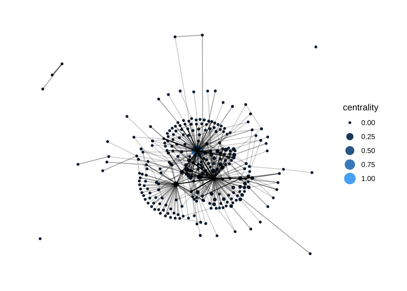

Figure 12.2: Network Graph with Centrality

There is much more you can do with {ggraph} (and {tidygraph}); check out the {ggraph} tutorial here: https://ggraph.data-imaginist.com/

12.8 Conclusion

In this chapter, we used social media data from the #tidytuesday hashtag to prepare and visualize social network data. Sociograms are a useful visualization tool to reveal who is interacting with whom—and, in some cases, to suggest why. In our applications of data science, we have found that the individuals (such as teachers or students) who are represented in a network often like to see what the network (and the relationships in it) look like. It can be compelling to think about why networks are the way they are, and how changes could be made to—for example—foster more connections between individuals who have few opportunities to interact. In this way, social network analysis can be useful to the data scientist in education because it provides a technique to communicate with other educational stakeholders in a compelling way.

Social network analysis is a broad (and growing) domain, and this chapter was intended to present some of its foundation. Fortunately for R users, many recent developments are implemented first in R (e.g., (R-amen?)). If you are interested in some of the additional steps that you can take to model and analyze network data, consider the appendix on two types of models (for selection and influence processes), Appendix C.